PostgreSQL partitioning is a powerful feature when dealing with huge tables. Partitioning allows breaking a table into smaller chunks, aka partitions. Logically, there seems to be one table only if accessing the data, but physically there are several partitions. Queries reading a lot of data can become faster if only some partitions have to be read instead of the whole table. Maintenance tasks will also benefit from the smaller partitions.
- first introduces the data used in the article and how to reproduce the examples,
- then explains partition pruning,
- finally shows range, list, and hash partitioning with PostgreSQL syntax.
Data preparation
First, pull and run the container with version 1.2 from a command line. Port 5432 is exposed, and you must set a password for the postgres database user.
And now prepare the data: create a table without partitions and without indexes and load sample data from spotify charts. The source data is available in the container in directory /usr/src/dwh_course/sourcedata.
CREATE TABLE ranking
(
rank integer,
track_id varchar(32),
artist_id integer,
no_streams integer,
url character varying(200),
stream_date date,
region character varying(10)
);
COPY ranking
FROM ‘/usr/src/dwh_course/sourcedata/spotify/ranking.csv’ DELIMITER ‘,’ CSV HEADER;
SELECT * FROM ranking LIMIT 10;
SET max_parallel_workers_per_gather = 0;
The screenshot shows the result of the three statements above. The created table contains the columns track_id and artist_id with foreign keys to data not used in this scenario. The data would be available in files stored in directory /usr/src/dwh_course/sourcedata/spotify/.
The table also contains columns for the data of the streaming (stream_date), the number of streams (no_streams), the region of the stream (region with values ‘de’ or ‘global’) and the position in the charts (rank). Finally, the URL points to the track.
Parallelism is switched off for better comparison of the explain plan outputs.

The base table is now prepared for the different partitioning scenarios. But why partitioning and not indexing?
Indexing for small data, partitioning for big data
Why is indexing not enough? There are access patterns that read “relatively” few rows only. Such access patterns work in most cases very well with indexes. But there are also access patterns that read many data (and might return many returns or aggregate the data into few returned rows). Indexes do not work well with such an access pattern. Database optimizers usually ignore indexes when retrieving many data. Alternative approaches like partitioning are the way to go. Partition pruning can help optimizing data retrieval.
Partition pruning
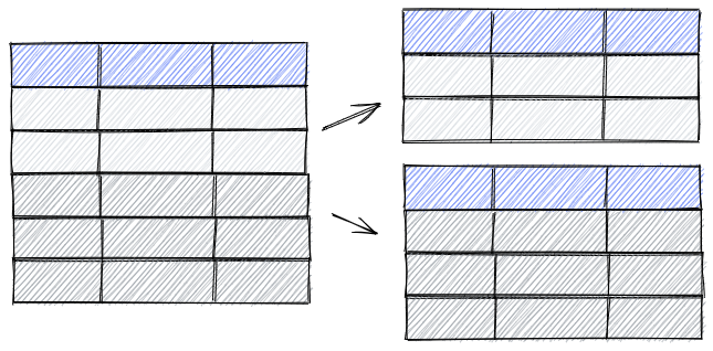
SQL statements can run faster if only some partitions have to be scanned in contrast to scan the whole table. Skipping irrelevant partitions is called partition pruning.
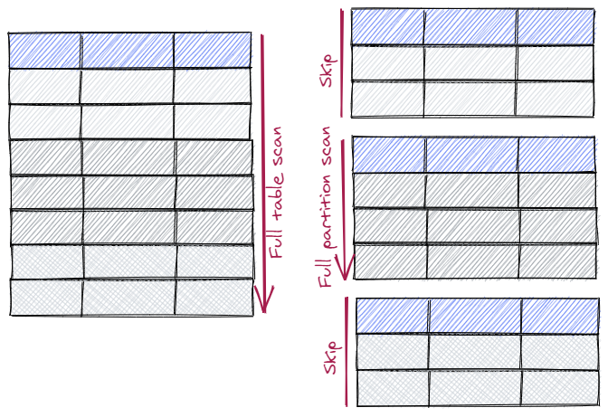 The picture shows a full table scan on the left. On the right is a partioned table. Instead of scannning the whole table, partition pruning skips some partitions while reading the remaining partitions. If the table is partitioned monthly by e.g. delivery_date column, only relevant months are read (e.g. a query with WHERE clause delivery_date = ‘15.01.2020’ will scan the partition for January 2020 only.
If a table is partitioned by delivery_date column and queries use order_date column in the WHERE cluase, partition pruning won’t jump in. The partitioning column need to be used e.g. in the WHERE clause.
Range partitioning
Range partitioning allows to specify ranges that are stored together. Typically date ranges are used, e.g. store data by year, by month or by date.
CREATE TABLE ranking_range
(
rank integer,
track_id varchar(32),
artist_id integer,
no_streams integer,
url character varying(200),
stream_date date,
region character varying(10)
) PARTITION BY RANGE (stream_date);
CREATE TABLE rank_2019 PARTITION OF ranking_range FOR VALUES FROM (‘2019-01-01’) TO (‘2020-01-01’);
CREATE TABLE rank_2020 PARTITION OF ranking_range FOR VALUES FROM (‘2020-01-01’) TO (‘2021-01-01’);
CREATE TABLE rank_max PARTITION OF ranking_range FOR VALUES FROM (‘2021-01-01’) TO (MAXVALUE);
INSERT INTO ranking_range
SELECT * FROM ranking;
ANALYZE ranking;
ANALYZE ranking_range;
The first part in the code block creates a range partitioned table. The sample data consists of the stream_date column. A date is a good candidate for range partitioning. Queries need to use the partitioning key to take advantage of partition pruning.
The following three commands create partitions for 2019, 2020, and default for values above. The partitions are by year. It would also be possible to partition by month or by day, depending on the specific requirements and access patterns. Partitioning several years by day will create many partitions – too many partitions can also cause performance challenges.
A common observation with range partitioning by date is the increase of rows. Data usually grows over time (e.g. sales) and therefore, the latest partitions contain more rows than older partitions. The sample data does not have this behaviour, though.
An insert fills the new ranking_range table, and the final statements compute statistics for ranking and ranking_range.
The following screenshot shows the code and the output of the statements.

EXPLAIN
select count(*)
from ranking
where stream_date between ‘2019-01-01’ and ‘2019-06-30’;
EXPLAIN
select count(*)
from ranking_range
where stream_date between ‘2019-01-01’ and ‘2019-06-30’;
The screenshot below shows the output of the explain statements. A full table scan is on the non-partitioned table, causing higher costs than the partitioned table. The partitioned table consists of three partitions (rank_2019, rank_2020, rank_max). A scan is only necessary on partition rank_2019.

List partitioning
List partitioning works with discrete values that can be enumerated like countries. List partitioning and multitenancy requirements are often combined.
CREATE TABLE ranking_list
(
rank integer,
track_id varchar(32),
artist_id integer,
no_streams integer,
url character varying(200),
stream_date date,
region character varying(10)
) PARTITION BY LIST (region);
CREATE TABLE rank_gl PARTITION OF ranking_list FOR VALUES IN (‘global’);
CREATE TABLE rank_de PARTITION OF ranking_list FOR VALUES IN (‘de’);
CREATE TABLE rank_default PARTITION OF ranking_list DEFAULT;
INSERT INTO ranking_list SELECT * FROM ranking;
ANALYZE ranking;
ANALYZE ranking_list;
The first part in the code block creates a list partitioned table. The sample data consists of the region column. The following three commands create partitions for the values ‘de’, ‘global’, and default. Queries need to use the partitioning key to take advantage of partition pruning.
An insert fills the new ranking_list table, and the final statements compute statistics for ranking and ranking_list.
The following screenshot shows the code and the output of the statements.

Now let’s compare the costs for a query against a non-partitioned and a list partioned table.
EXPLAIN
select count(*)
from ranking
where region = ‘de’;
EXPLAIN
select count(*)
from ranking_list
where region = ‘de’;
The screenshot below shows the output of the explain statements. A full table scan is on the non-partitioned table, causing higher costs than the partitioned table. The partitioned table consists of three partitions (rank_gl, rank_de, rank_default). A scan is only necessary on partition rank_de.

Hash partitioning
Hash partitioning works by specifying a modulus and a remainder.
CREATE TABLE ranking_hash
(
rank integer,
track_id varchar(32),
artist_id integer,
no_streams integer,
url character varying(200),
stream_date date,
region character varying(10)
) PARTITION BY HASH(artist_id);
CREATE TABLE rank_h0 PARTITION OF ranking_hash FOR VALUES WITH (modulus 3, remainder 0);
CREATE TABLE rank_h1 PARTITION OF ranking_hash FOR VALUES WITH (modulus 3, remainder 1);
CREATE TABLE rank_h2 PARTITION OF ranking_hash FOR VALUES WITH (modulus 3, remainder 2);
INSERT INTO ranking_hash
SELECT * FROM ranking;
ANALYZE ranking;
ANALYZE ranking_hash;
The first part in the code block creates a hash partitioned table by using the artist_id column. The following three commands create three partitions with modulus three and remainder 1,2, or 3. Queries need to use the partitioning key to take advantage of partition pruning which can become very difficult or even impossible with hash partitioning. Therefore, hash partitioning is mainly used to distribute data and to avoid hot spots.
An insert fills the new ranking_hash table, and the final statements compute statistics for ranking and ranking_hash.
The following screenshot shows the code and the output of the statements.

Now let’s compare the costs for a query against a non-partitioned and a hash partioned table.
EXPLAIN
select artist_id, count(*)
from ranking
group by artist_id;
EXPLAIN
select artist_id, count(*)
from ranking_hash
group by artist_id;
The screenshot below shows the output of the explain statements. There are full scans on the non-partitioned table and on the partitioned table. The cost of the hash partitioned table is even higher due to overhead. The SQL statement does not use the partitioning column. But there is an alternative approach to writing the query to take advantage of hash partitioning and decrease the costs.

The screenshot below shows an alternative approach. The SQL statement is written with a union combining the results of three sub statements querying a hash partition. The resulting explain plan shows much lower costs compared to the original statement against the partitioned table.

Summary
The article explains different partitioning scenarios for PostgreSQL. The main advantages of using partitioning are:
- Improve performance for queries accessing many rows.
- Easier administration, e.g. if you reorganize table partitions to different tablespaces with faster and slower disks.
- Reduce hot spots by spreading changes (inserts, updates, deletes) across partitions.